Increase Efficiency

This report covers the project’s goal to increase the efficiencies of the heating system that feeds the district heating network (DHN). In previous sections, energy demand and energy supply were described. Here, first a system analysis is presented. This is followed by the data analysis and strategy generation. After the modelling is described, the results are presented. In the conclusion, further work is described.

System Analysis

For the system analysis, first the insights from the energy supply section were condensed and concluded. This was followed by the analysis of the environmental and financial benefits for the University.

Condensed Insights from Energy Supply

The system analysis carried out points to low efficiencies of both, combined heat and power scheme (CHP) as well as boilers. In 2021, the CHP reached a total efficiency (as the ratio of useful energy compared to fuel input) of 66% (see Figure 1). Published benchmarks suggest 80% can be achieved (EPA not dated) and will later be shown to potentially reach 86% (Vital Energi 12/2021). The manufacturer of the boilers was contacted and they provided technical documentation that claims the expected efficiency to be as high as 97% (Worcester, Bosch 08/2020). This led to the conclusion, that efficiencies could be increased by 30% and 43% for the CHP and boilers, respectively.

Figure 1: System analysis (left) and efficiencies compared to benchmarks (right).

Environmental Benefits of the CHP for the University

In the past, the CHP helped the University to decarbonise its system. The UK Department for Business, Energy & Industrial Strategy (BEIS) publishes the applicable carbon emission factors yearly (BEIS 2010-2021). This is compared to three possible sets of CHP efficiencies (see Figure 2) where the red line represents the current system, the yellow line is the proposed system, and the green line is the typical efficiencies for commissioning (shown are total and electrical efficiencies) (EPA not dated). Thus, the grid electricity became less carbon intensive than the current set-up in 2018. The commissioned system would still be helping decarbonisation in 2021.

Figure 2: Carbon emission factors of electricity from grid and differing CHP efficiencies.

Financial Benefits of the CHP for the University

The University benefitted and still benefits from the CHP in a financial sense, as will be shown in this subsection. There is a significant spread between gas and electricity prices. Below, the current system is illustrated (see Figure 3). For an input of 3 kWh of gas, 1 kWh of useful thermal and electrical energy can be harvested.

Figure 3: Exemplified harvest of the CHP using 3 kWh of gas input (current system).

Using prices applied in 2020 and 2021, as well as efficiencies derived for the CHP (WSP 12/3/2021) and the boilers feeding the system before 2018 (SIA 384/3), the overall comparable cost was derived (see Table 1). The CHP therefore helps the University in saving money thus having its financial benefits.

Table 1: System and price comparison, old/new system and 2020/2021.

As an additional aspect, the CHP’s lifespan is expected to be around 15 years (EN 15459:2007; SIA 384.110). After this initial analysis, it seemed worthwhile to further analyse how to unlock the CHP’s full potential.

Data Analysis

For data analysis, first a curated dataset needed to be extracted. This was followed by analysis of the CHP efficiencies and concluded by the analysis of boiler efficiencies.

Used Dataset

The data analysis was based on half hourly metered readings for the year 2020 (Strathclyde Real Estate 2022). February 29 was excluded to get a standard dataset of 8’760 h/a with 17’520 datapoints. Available heat meters were analysed, and a schematic drawn (see Figure 4). Electricity data was available in daily readings, therefore with a differing temporal resolution. As a work-around, an electricity profile for the University of Strathclyde in adequate resolution was used based on consumption 2011 (ESRU 2022). This was sized to meet the demand of the year 2021 in a curation process (WSP 12/3/2021).

Figure 4: Available heat meters for analysis.

Analysing CHP Efficiencies

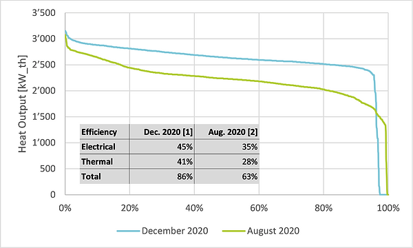
The analysis to generate a strategy to cure missing CHP efficiencies, required the above-described dataset to be converted to supply duration curves (see Figure 5). The comparison is based on a summer month (August) and a winter month (December) of the year 2021. The efficiency data was taken from data available for the year 2020 (Vital Energi 08/2021, 12/2021). The CHP often ran close to its rated power in December. The overall efficiency increased from 63% to 86% from August to December, respectively. The analysis of all meter readings showed hardly any datapoints above 3 MW. Therefore, further analysis was based on 3 MW as rated maximum heat output.

Figure 5: Supply duration curve for December and August 2020 including efficiencies.

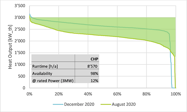
Further analysis showed that overall, the CHP reached a very high runtime and availability of 8’570 h/a and 95%, respectively. The CHP reached the rated heat output only during 12% and operates 78% of the runtime in part-load.

In conclusion, the analysis indicated significant potential, depicted by the green area below (see Figure 6). This potential lies idle, and a new system may strive to unlock it to its maximum.

Figure 6: Unused potential: Difference between assumed power and generated heat.

Analysing Boiler Efficiencies

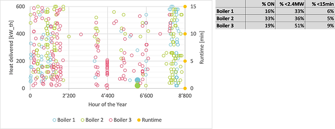
The analysis to generate a strategy to cure missing boiler efficiencies was based on the same dataset. The poor performance of the boilers was attributed to the control strategy applied. Analysis showed that often two boilers were operated at the same time. This was true for loads when the runtime for one boiler would lie below 15 min (see Figure 7). The annotation around the 6000th hour of the year shows two boilers were turned on for about a minute each (at the same timestep, see green/blue filled circle).

Further examination showed low runtimes. This was not surprising, since the overall installed capacity (i.e. 27.3 MW) surpasses the demand (max. 14.6 MW in 2020) by a factor of nearly two. This could be explained by concerns of security and redundancy. In addition, the system was designed to be expanded (e.g. Strathclyde’s Halls or the City Chambers).

During their operation, boilers were run at one third (33%) to more than half (51%) their runtime for less than an hour continuously. They even did not reach a steady 15 min for 5% to 9% of being switched on. In conclusion, this analysis indicated the need to explore alternative control mechanisms to guarantee longer continuous and efficient hours of operation.

Figure 7: Scatterplot of operational data for 2020, circles representing heat delivered.

Strategy Generation

The newly generated strategy was built upon the findings of system and data analysis. The aims were (i) to explore how the CHP could be used as financial asset, (ii) apply changes to reach a higher CHP output, and (iii) to allow for longer continuous boiler operation times.

To achieve this, essentially three things were changed (see Figure 8). First, boilers were only allowed to cut in at 30% of their rated power. Second, the CHP was run to its maximum capacity whenever possible resulting in the need to sell excess electricity behind meters (see below). Third, due to the surplus heat generated by the CHP the tripling of the volume of the current thermal energy storage was required. This measure was based on a parameter study to find the optimal size.

The peer-to-peer sales of surplus electricity behind the meter using a private line was assumed to be a realistic possibility. For this case study, the City Chambers were assumed to act as peer benefitting from the same conditions as the University (20 p/kWh_el). The advantage of this assumption is that the University either saves money when not buying electricity from the grid or gains money from selling. Thus, uncertainties of the electricity demand profiles could be eliminated.

Figure 8: Schematic of the new system and the changes marked in red.

Modelling

The modelling relied on the dataset used for data analysis as well as further assumptions from system analysis, literature review, and was influenced by insights from the analysis of Strathclyde’s Sustainability reports. In this section, the applied control strategies are discussed, followed by the description of the method used in the modelling process. Subsequently, the method of implementing the heat and electricity balance is shown as schematics (and provided as ‘code’ in Annexes in the full report, see More > Resources).

Control Strategies

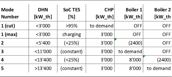
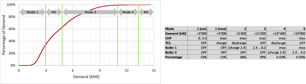
Accounting for the changes proposed and following the aims for the new system, which were based on the system and data analysis, control strategies needed to be derived. The implemented control strategies were based mainly on heat demand and management of thermal energy storage (TES). For simplicity, the demand of the district heating network (DHN) is assumed to be known to the supply system. This was implemented in the model and is true since the case study could be based on 2020 demand data. This ultimately led to five modes, one of which comprised two sub-modes (see Table 2). Modes were defined solely based on the demand of the DHN. The CHP and boilers were further controlled to meet the demand (1, 3, 5), and in three modes (1, 2, 4) by the state of charge (SoC) of the TES.

Table 2: Control strategies as modes depending on demand.

Modelled Recursive Energy Balance

These rules were implemented in a recursive model using an energy balance set up in Excel. ‘Recursive’ means certain decisions made relied on the last timestep (i.e. half an hour). ‘Energy balance’ means that supply data was processed and heat losses and losses due to stratification were excluded.

We expect that in the field a similar result as suggested could be achieved. CHP and boilers could be controlled solely according to charging and discharging velocities in the enlarged TES. ‘Dis/charging velocity’ means that evenly placed thermal sensors could be used to derive the time needed to reach changes between two adjacent sensors. Hence lost/gained capacity could be calculated. An additional advantage of this approach was that losses and stratification automatically were considered and smaller timesteps could be achieved. This would be dependent on the implemented building energy management system where readings more frequent than half an hour are not uncommon.

Modelled Heat Balance

The modelled heat balance of all five modes and two sub modes can essentially be broken down to four different heat balances (see Figure 1). Top left, the CHP directly feeds the DHN to its demand since the TES is fully charged to 90%. Top right, the surplus energy from the CHP is stored, i.e. the TES is charged (floating between 25% and 90%). Bottom left, the TES is discharged and once falling below 25% SoC will be supported by the boiler at its cut-in power of 2.4 MW. For higher demand, boiler 1 runs at maximum capacity and boiler 2 is charging the TES (this is mode 4 as opposed to mode 2). Bottom right, the boilers cover the surplus need of the DHN (in mode 3: only boiler 1; in mode 5, when boiler 1 runs at maximum, boiler 2 covers the surplus).

Figure 9: Schematics of the heat balance used as heat flows.

Modelled Electricity Balance

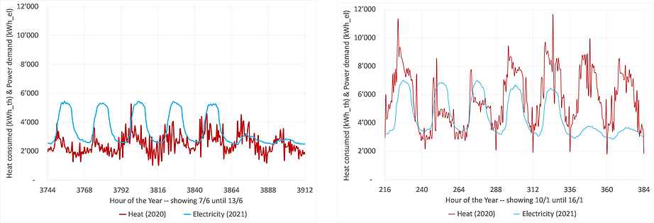
The electricity imports omitted, and exports sold, respectively, are calculated by using the half hourly demand profiles (see two examples for Summer and Winter, respectively in Figure 10). Here, electricity demand is much smoother than metered heat data. There is metered data for electricity, but not in the temporal resolution of half an hour. Therefore, electricity profiles of the year 2011 (ESRU 2022) were adjusted to metered demand of the year 2021 (WSP 12/3/2021). As described above, assuming the same price for imports and exports was the chosen approach to eliminate possible errors.

Figure 10: Half hourly demand profiles for a week in Summer (left) and Winter (right).

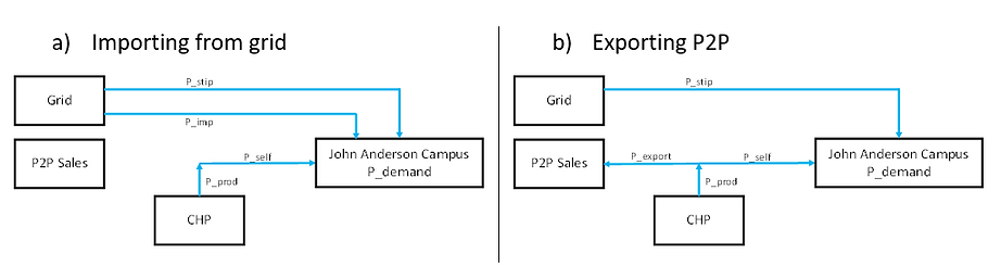
The electricity balance essentially starts with demand from which the imports as stipulated by contract are subtracted. The power generated by the CHP as a priority is self-consumed. If the production is not enough to cover demand, needed electricity is bought from the grid (see Figure 11 a). If the production is too high, it is exported. (see Figure 11 b).

Figure 11: Schematic of the electricity balance, left importing and right exporting.

Results

Certain parts of the results led to iteration loops within the modelling section. Therefore, first the parameter study of sizing the TES is described, followed by the results for the different operational modes, the technical results, the changes in carbon emissions, and finally the financial consequences.

Parameter Study of Sizing the TES

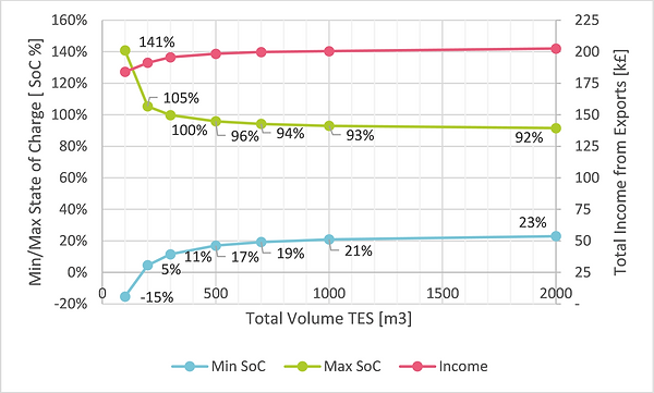
To find an optimal size of the TES, a parameter study was carried out. Total size of TES using the model above was calculated for values ranging from 100 m³ (as is) to a maximum of 2’000 m³ (see Figure 12). The work focussed on two aspects. First, technical aspects, which needed to be met. Second, a KPI to help the decision-making process which TES would be likely to be optimal.

On the technical side, (i) the minimal SoC should not fall below zero since this would lead to a shortfall of meeting the demand. (ii) the maximum SoC should not be higher than 100% since this would possibly lead to safety issues because supply exceeded demand leading to rising temperatures of the system. As KPI, the total of savings and earnings of the achieved electricity production was used. Note, gas consumption for all sizes was analysed and shown to stay close to constant for all sizes with 0.2% higher demand for 2’000 m³ than the base-case, 100 m³.

Figure 12: Parameter study to size the thermal energy storage (TES).

There are three sizes fitting the definition of an ‘optimum’. (i) doubling the TES led to slight overshoot with a max. SoC of 105%. This might still be a valid option accounting for thermal losses and losses due to stratification. On a technical side, shorter time steps for control could possibly be used as solution. (ii) tripling the size met all criteria and was further used in the model. (iii) further enlarged volumes such as 500 m3 worked as well but could not be proven to offer additional benefits. On the contrary, their massive size might even threaten the project. Concerning space demand, spare space put aside for a second CHP in the energy centre (EC), or the courtyard next to it, offered potential for the integration of additional TES capacity.

Relevance of the Different Operational Modes

The results of the overlap of the different heating modes with the duration curve showed that in the year 2020 modes 4 and 5 were not of real importance (see Figure 13). The changes of this new control approach mostly applied to modes 1 and 2 which accounted for 71% of the system’s total runtime. In mode three (29% of the year), only one boiler ran at any given time. This boiler could be any given boiler which will be run using operating time equalisation.

Figure 13: Modes 1 to 5 applied to the duration curve of demand in 2020.

Requirements for P2P Sales

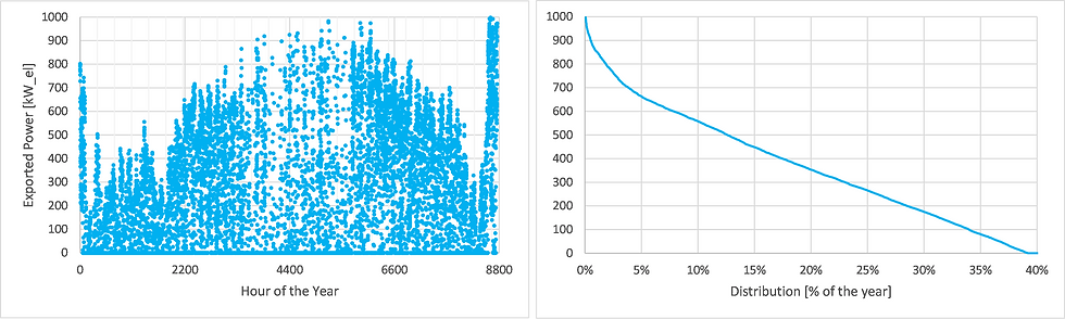
Potential partners for peer-to-peer (P2P) sales should be able to take as much as 1’000 kW_el (see Figure 14). The suggested scheme would lead to sales during 40% of the year and a quite scattered delivery pattern. Highest delivery would be in winter, whilst in summer some peaks are encountered but in between there are just as many missing hours without delivery.

Figure 14: Scatterplot of electrical power exports and power distribution.

Technical Results

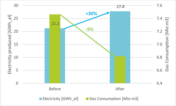
The technical results compare the “before”, i.e. the situation now with 100 m³ TES, to the situation “after”, i.e. the optimised size of 300 m³ TES (see Figure 15). Accounting for the benchmark efficiencies, overall electricity production could be increased by 30%. At the same time, gas consumption could be decreased by 9% although intuition expected an increase. This may be explained by the massive increase of the CHP’s efficiency from 66% (before) to 86% (after) where the gas input generates 30% more useful energy output.

Figure 15: Electricity produced and gas consumption before and after.

Changes in Carbon Emissions

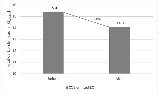
In terms of carbon emissions only gas reduction was considered. The increase of energy production and substitution of grid electricity was scoped out since there are differing predictions available (ICAX not dated; NationalGridESO 2021). The reduction accounted for a total of 1’330 t/a (see Figure 16). The CHP scheme still emitted 14 kt/a and therefore, exceeded the targeted CO2 budget of the University for the year 2030 of 6 kt/a more than by a factor of two.

Figure 16: Carbon emissions of the Energy Centre (EC) before and after.

Financial Consequences

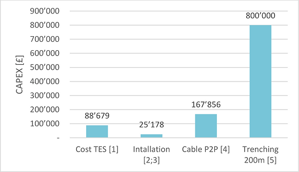
In terms of financial results, the cost for the additional TES (FLEXYNETS 2019), its installation and integration (H. Gmür 3/15/2022; K. Hildebrand 3/15/2022), the needed cable for peer-to-peer (P2P) sales (V. Wouters 3/15/2022), and the trenching from the EC to the City Chambers (D. Charles 3/23/2022) were accounted for (see Figure 17). The total CAPEX thus amounted £ 1.1 Mio where trenching takes the biggest share. This is supported due to knowledge of costs during the installation of the DHN.

Figure 17: Investment cost for TES, installation, cable peer-to-peer, and trenching.

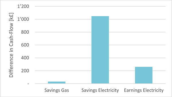
This is contrasted by savings due to reduced gas consumption and omitted grid imports supplemented by earnings from electricity sales (see Figure 18). For a total lifespan of 25 years, an interest of 5%, the energy prices for gas at 5 p/kWh, electricity import/export equal at 20 p/kWh total savings/earning added up to £ 1.3 Mio/a. This led to a payback time of less than a year. Ultimately, the CO2 abatement cost reached £ 58/t_CO2e.

Figure 18: Cash-flow due to savings and earnings.

Conclusion

This case study illustrates how a system can be run closer to its optimal efficiency by the integration of larger thermal energy storages. The work is based on metered, half-hourly data and the suggested control strategy may be adapted to be included into any building energy management system reaching even higher temporal resolution and leading to smaller thermal energy storages. This needs further investigation which ultimately might show that doubling instead of tripling thermal energy storage may suffice. Phenomena such as heat losses and losses due to non-optimal stratification could be included in this work. A better understanding of savings vs. earnings from generating power could be reached using metered data of electricity in the same temporal resolution as heat. Thus, phenomena of differing prices (import vs. export) could be researched. In addition, a sensitivity analysis of efficiencies before and after might lead to insights of parameters of the highest leverage. In this process, the assumed electricity efficiency of 45% should be scrutinised since the value seems high.

Concluding, the above-described approach seems to be worth further pursuit and depends on three changes. First, adaptions in control for boilers can be implemented immediately (very short term). Second, the installation of additional thermal energy storage capacity is dependent on the space for installation but could possibly be realised inside the energy centre using spare space put aside for the installation of a second combined heat and power scheme (short term). Following, the existing combined heat and power scheme could start to run at higher capacity (short term). Its maximised capacity depends on solving this third point: assuring a partner for peer-to-peer sales of surplus electricity generated. This search can start immediately and will ultimately be crucial to how fast trenching can be done considering distance and the complexity of underground (short to midterm).

Acknowledgements

David Charles for invaluable support both in providing data, granting access to internal reports, and keen interest as well as weekly support to the cause.
Neil McBeth for the virtual tour around campus.
Paul Tuohy for sending the ESRU data at a time when the website was down.
Harry Gmür, Kurt Hildebrand, and Volker Wouters for providing investment data.

References

BEIS (2010-2021): Government conversion factors for company reporting of greenhouse gas emissions. Department for Business, Energy & Industrial Strategy. Available online at https://www.gov.uk/government/collections/government-conversion-factors-for-company-reporting, checked on 1/31/2022.
D. Charles (2022): Pricing of Trenching. via Zoom to St. Mennel, 3/23/2022.
EN 15459:2007; SIA 384.110, 6/1/2008: Energieeffizienz von Gebäuden [Energy Efficiency of Buildings].
EPA (not dated): CHP Benefits. Available online at https://www.epa.gov/chp/chp-benefits, checked on 5/7/2022.
ESRU (2022): Demand Profile Database. due to Paul Tuohy.
FLEXYNETS (2019): Large Storage Systems for DHC Networks. Fifth generation, low temperature, high exergy district heating and cooling networks. Available online at https://w4u0es9f4.wimuu.com/Download?id=file:68931000&s=5624676745098706070, checked on 3/15/2022.
H. Gmür (2022): Pricing of TES Integration - System. via phone to St. Mennel, 3/15/2022.
SIA 384/3, 2020: Heizungsanlagen in Gebäuden - Energiebedarf [Heating Systems - Energy Demand].
ICAX (not dated): Grid Carbon Factors. Available online at https://icax.co.uk/Grid_Carbon_Factors.html, checked on 2/23/2022.
K. Hildebrand (2022): Pricing of TES Integration - Controls. via phone to St. Mennel, 3/15/2022.
NationalGridESO (2021): Electricity Ten Year Statement. Available online at https://www.nationalgrideso.com/research-publications/etys, checked on 4/21/2022.
Strathclyde Real Estate (2022): Half-hourly metered Heat Data. due to David Charles.
V. Wouters (2022): Pricing of Cabling (1,200 MW). via phone to St. Mennel, 3/15/2022.
Vital Energi (08/2021): Operational Report - August. internal report to Estates.
Vital Energi (12/2021): Operational Report - December 2020. internal report to Estates.
Worcester; Bosch (08/2020): Technical and Specification Information.
WSP (12/3/2021): UoS Sankey Diagrams – Technical Note (Confidential Report). internal report to Estates.