The most effective approach that enables campus buildings to lower their corresponding CO2 emissions can be achieved by implementing retrofitting measures. The energy performance of a building can be optimised through retrofitting, resulting in a decrease in energy demand and thus CO2 emissions. By investing in retrofitting campus buildings, The University of Strathclyde will be moving in the right direction in meeting their emission targets. According to the International Energy Agency (IEA) statistics and energy balances, it was concluded that in 2014 the building and construction sectors consumed a total of 122 exajoules, contributing 30% to the total global final energy use (Dulac.J 2016). In addition, from a research analysis performed by Yuamming, it was presumed that on average, the rate of heat loss from a building envelope, through its constructions such as external walls, roof and floors were 62%, 19% and 7% respectively (Kwan.Y, 2015). Heat transfer mechanisms such as conduction, convection, radiation, and mass transfer are the contributors to these losses, which are caused due to poor or even uninsulated surfaces, and due to the improper selection of construction materials resulting in higher energy losses. Therefore, retrofitting measures such as optimisations to the building envelope constructions and energy management schemes should be established, to be able to reduce the rate of heat loss and hence increase the energy efficiency of the building by lowering its demand. For this strategy, one building in the John Anderson campus was chosen as a case model to assess the effect of retrofitting buildings. 

​

Methodology

​

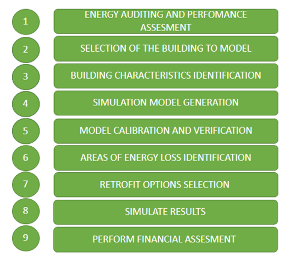
For this strategy, a series of steps were considered to be able to undertake this assessment and are summarised below.  

​

​

​

​

​

​

​

​

​

​

​

​

 

 

 

 

 

 

 

​

 

Case model 

​

For this study, the building chosen to simulate was Thomas Graham, located on Cathedral Street. It has in total eight floors with a gross floor area of 14,594 m², according to the data provided from the estates department. The building belongs to the department of Chemical and Process Engineering, which accommodates different types of rooms such as classrooms, lecture theatres, laboratories, and research rooms.   

Thomas Graham (TG) was selected due to its high energy use intensity compared to other buildings in the campus. As it can be seen from table 1, TG has the highest annual heating energy use intensity with a value equal to 214 kWh/m². According to the CIBSE guide F: Energy efficiency, a typical benchmark for a building with similar functionality as TG should be around 110 kWh/m² (CIBSE, 2020). The difference between these two values indicates that there are areas in the building where heat energy is being lost, hence the need for retrofit measures to be established.  

​

Table 1: Energy use intensity for various buildings in the campus

 

 

 

 

 

 

 

 

 

 

                                                                      

Building energy simulation software

 
To be able to evaluate the energy performance of Thomas Graham an engineering building simulation tool was used called ESP-r. It is a modelling tool that was created by the University of Strathclyde and can effectively calculate the energy performance using a finite volume procedure. ESP-r can model different functions that consume energy in a building, such as heating, cooling, and electrical power for appliances (Strath, 2022). This software was chosen as an ideal tool for this analysis, since it has several capabilities such as the ability to simulate models at different time-steps, it can apply a heat balance to each individual zone of the model, and it is user friendly nature. 

​

Current energy consumption 

 

Based on the heat metered data provided by the Energy System Research Unit (ESRU), different energy profiles were able to be generated for Thomas Graham and are represented on figure 1.  

​

​

​

​

​

​

​

​

​

 

 

 

      Figure 1: Comparison of energy use intensity and average heating degree days for 2019 and 2020.

 

The bar chart shows the annual heating demand for 2019 and 2020 and the line graph details the average heating degree days by dotted lines. The average values for heating degree days were gathered from the website of the government (GOV.UK, 2021). Taking into consideration the average heating degree days for both years, it was concluded that 2019 had higher heating degree days than 2020 which explains the fact that the annual heating demand for 2019 was higher. In 2019 and 2020 the total heating consumption of Thomas Graham was 3.4 GWh and 3.1 GWh respectively. In more depth, during the summer period between June and August, it was identified that the energy use intensity was relatively high, which suggests that the building is either poorly insulated or there was internal consumption in labs or research rooms which require special conditions to operate. Therefore, the whole building was modelled to simulate the current energy consumption and then implement retrofit measures that would improve the energy performance of the building resulting to a lower heating demand.  

 

Thomas Graham building has a total gross floor area of almost 15,000 m². For this project, only part of the building was modelled, the bottom part of level 2, which is represented by the red box on the floor plan on figure A1 in the appendix. To be able to model the building, dimensions were gathered from the floor plan and by visual inspection. From the visual inspection of the building, it was identified that there are several rooms with varying functionalities. For example, there are rooms that are lecture theatres, research rooms, and others that are laboratories. Hence, due to their variety, it was ensured that each room was assigned as a different thermal zone with distinct operational details. This extra parameter enabled the model to be more accurate in representing the real conditions. 

The base model geometry was constructed in ESP-r and is shown on figure 2. The model dimensions, floor areas, internal volumes, and window sizes were assigned as per the floor plan and from a real-life measuring of the existing rooms of the building.

​

​

​

​

​

​

​

​

​

​

​

​

​

 

                                                                Figure 2: Modelled geometry of Thomas Graham

​

​

The total surface area of the model was found to be 820 m² consisting of five different rooms connected to each other by a large corridor. To be able to run the simulation and generate initial results the model was assigned with specific operational details and each construction with varied materials. Full details of the model and its zones (including construction details, material properties, geometrical properties, heat gains, and operational performance) can be found in the pdf file down the bottom of this page as a link.   

 

 

Assumptions and simplifications

​

While constructing and simulating the model different assumptions and simplifications were used and can be seen below:

•    While constructing and simulating the model different assumptions and simplifications were used and can be seen below:
•    The whole simulation was based only on the heating energy consumption since the data provided were half-hourly heat metered                data. 
•    The air mixture infiltrating the building was assumed to be well mixed with a constant temperature.
•    The building is open from 8am till 18pm, therefore the heating system was scheduled to begin operation from 7am so that the rooms          are heated before any users start to enter the building.  
•    All the heat transfer that occurred in the model was accounted to be one dimensional. 
•    The operational details, such as heat gain by occupants, equipment, and lighting were gathered from CIBSE Guide A chapter 6                (CIBSE, 2015). 
•    The heating load was only sensible heat therefore there were no latent heat loads considered and hence, no control on the relative            humidity. 
•    The multiple windows in each room were combined to form a bigger one with the same area and from that area it was assumed that          15% represents the framing. 
•    The roof and the floor of the model were assigned adiabatic boundary conditions, meaning that there was no heat transfer                          mechanism taking place. 

​

Model calibration and validation 

​

After the generation of the geometry, the model was assigned with all the relevant boundary conditions and specific materials, to be able to run the model and deduce the estimated heating consumption from the software. The graph below (figure 3) shows the monthly heating consumptions for the original building data plotted against the data generated from the simulation.

 

 

 

 

 

 

 

 

 

 

 

Figure 3: Heating consumption of simulation results vs theoretical original data from half-hourly data

 

For the two data sets to be comparable, the energy use intensity for each month (using the heat metered data) was calculated based on the total heating consumption per month, which was divided by the gross floor area of the building. Then the modelled geometry total gross floor area was multiplied with the EUI mentioned above to deduce the theoretical heating consumption of the building. The following section demonstrates a sample calculation used to calculate the theoretical consumption.

Sample calculation

January 2020: Heating consumption from half-hourly data was equal to 356.7 MWh. Hence,

​
 

​

Model geometry total gross floor area was equal to 820m². Therefore,

​

​

​

From the chart above it was identified that the model underestimated the heating consumption. It was determined that this was mainly due to energy losses in the roof and floor that were not considered by the modelling tool. The main reason for this was, that the two construction boundary conditions were set as adiabatic, which implies that there is no heat transfer occurring. In a real-life situation this is not feasible and hence several changes were made to the model to account for this difference. Furthermore, another important fact that was deduced from this bar chart was the relative high heating consumption during the summer period which indicates that either the building is poorly insulated or there is heating energy consumed internally in labs or research rooms. 
Therefore, to be able to estimate the internal heating consumption, a simple analysis was performed to calculate the average yearly base load based on the data from the chart and was found to be approximately 6 MWh per month. By optimising the model to accommodate for this difference, the model was run once more to deduce of final percentage error of ±16.7%, which suggests that the model can provide a reasonable estimation for the total heating consumption. 

 

Results and Discussion

​

After the final model was calibrated and validated, the simulation was run to deduce the original energy consumption of the model before any retrofitting optimisation measures were adapted. The total annual energy consumption of this section of the simulated building came out to be 86.7 MWh. Since the main aim of this strategy was to increase the energy efficiency of the building, an extensive analysis was performed to determine the main areas of the building that contributed to the loss of heat energy. As a result of the analysis, it was concluded that heat was lost due to conduction and convection through the externals walls and the windows. Therefore, changes to windows configuration and improvements to the insulation level to all the external and internal walls were considered to lower the heating demand and hence reduce the average EUI per annum to the typical benchmark provide by CIBSE of 110 kWh/m². To be able to achieve this target, retrofitting standards such as PAS2038:2021 were considered. These standards refer to retrofitting strategies for non-domestic buildings for improved energy performance and provide specific target values . For example, the U-value that must be achieved for all the external walls should be around 0.15 W/(m²K) and for the windows the U-value must be lower than 0.8 W/(m²K). 

 

Insulation level optimisation

​

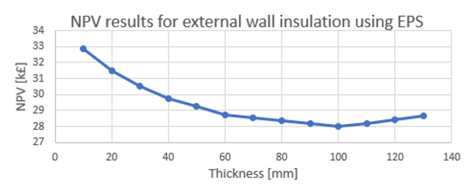
According to literature, some of the most widely used insulation materials are glass wool, polyurethane, and expanded polystyrene (EPS) and their thermal conductivities are 0.035, 0.025 and 0.03 W/mK respectively, accounting for 80% of the insulation materials used [6,7]. For this investigation the insulation materials used were glass wool, grey EPS, and polyurethane boards. Different thicknesses were used to deduce the overall heating consumption of the model after their implementation. Since cost was another key performance indicator, an extra analysis called Net Present Value (NPV) was used to identify the optimum thickness of insulation for each material tested, that would result in a lower heating consumption, considering a specific payback period of 45 years. Finally, the three materials mentioned above, were used to examine their performance for different type of constructions such as external and internal walls. The following graph represents an example from the results of the NPV analysis used to determine the optimum thickness of insulation material for the external wall. . 

 

​

 

 

 

 

 

​

                                                         

 

Figure 4: Net present value analysis for external wall using expanded polystyrene.

 

From the graph it was deduced that the optimum thickness for insulation for the external walls would result in the maximum demand reduction, while also considering cost, is 100 mm insulation. The following table summarises the results from the NPV analysis with the suggested optimum thicknesses for external and internal walls.

​

                                           Table 2: Results for optimum thickness of insulation on the external and internal walls.

​

 

 

 

The final step was to identify the insulation material that, based on the optimum thickness deduced above, would achieve the highest heating demand reduction. The table shows the three different materials with their corresponding heating demands when they were implemented in the model. 

 

Table 3: Heating demands achieved with different insulation material assessed.

 

 

 

 

​

 

From the above results, it was concluded that the most suitable material for insulating the external walls would be grey expanded polystyrene since, as seen from the results, it is the most cost-effective material that resulted in lowering heating demand. In the same manner, the most suitable material for insulating the internal walls was found to be glass wool.

​

Window optimisation

​

Another key aspect that was considered when optimising the energy performance of the building envelope, was glazing. Window glazing configuration highly contributes to the heat losses which, according to Energy.gov can reach a percentage of over 25%  (Energy.gov, 2022). Therefore, energy efficient glazing, such as double or even triple glazing, can effectively reduce the heating consumption of any building. Features such as glass type and gas gap materials should be considered, as well as their corresponding configuration with layer thicknesses, when deciding which glazing type to incorporate. Considering the BS EN 14351 and the Building Regulations 443, the glass used to configure the glazing should have a U-value no greater than 1.6 W/m²K and a thickness in the range from 4 to 6 mm. Usually, the gaps between the two panels of glass should be filled with air or any inert gas such Argon or Xenon. Argon and Xenon are denser gases than air, which result in higher energy efficiency of the window due to lower internal convection. In addition, Argon and Xenon, due to their densities, provide an additional benefit of not allowing the two glazing panels to stick together, consequently reducing the performance. Moreover, Argon and Xenon are inert gases, which means that there is no moisture content and hence it could result in a lower thermal conductivity of about 67% compared to air (TWS, 2021). Therefore, standards and building regulations were considered, and thus different configurations and compositions of glazing types were tested to deduce the optimum that would result in a lower heating consumption. The table at the bottom summarises all the results from this assessment and they were used to identify the optimum window configuration that would result in lowering the heating consumption.

​

                   Table 4: Building heating consumptions with different window configurations using different separation gas in the gap.

 

 

 

 

 

 

 

 

 

From the results it can be clearly seen that Argon can significantly reduce the heating consumption of the building and thus was chosen as the separation gap gas. Hence from the results, the optimum configuration was found to be 6 mm glazing thickness both internally and externally, with an Argon filling resulting in a total thickness of 20 mm. 

​

Building energy management system (BEMS)

​

Apart from optimisations to the building envelope such as insulation levels and glazing, the other area that has equal importance is how to manage the energy consumed in the building. BEMS are extensively used in new buildings, with their main function being to monitor and control the useful energy use in the building services such as air-conditioning systems, heating, lighting, and the power consumed by equipment. According to CIBSE, properly implemented BEMS can result in a 15-20% reduction in the annual energy consumption (CIBSE, 2015). This methodology is a cost-effective way of controlling energy consumption since it has an overall cost of £50 per square meter and a relatively short payback period of 3-4 years (Cheng. C, 2018). 

 

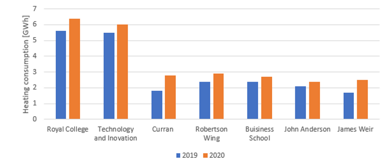
From a simple investigation on the energy profiles of various buildings on the campus, it was identified that there is lack of BEMS. In March 2020, the entire world was faced with the COVID-19 pandemic and hence, people were forced to stay at home. This meant that there should be no occupancy in the buildings of the campus. This would suggest that the energy consumption should fall, but instead the energy almost stayed unchanged. Figure 5 represents the energy profiles of different buildings across the campus prior to the pandemic 2019 and 2020 during the pandemic. 

 

​

 

 

 

 

 

 

 

 

                                                                   

 

   

 Figure 5: Prior and during COVID-19 heating consumption data.

 

From the graph it was clearly deduced that the overall heating consumption in the buildings increased rather than decreased as expected due to the pandemic. This increase in energy consumption was based on the fact there was no occupancy in the buildings which suggests that there were no associated internal heat gains resulting in higher consumption. By excluding this parameter, it was identified that the heating supply to the building was almost unchanged which implies that the university has no building energy management schemes to control these changes in demand. 

 

Proposed change:

The implementation of an effective BEMS should be considered by the university since it can reduce the energy consumption of buildings and hence increase the energy efficiency. This could be achieved by the implementation of various hardware such as occupancy control sensors, motion sensors for lighting, and thermostats at different control zones that will be connected to a controller. The controller would receive the recorded signals from the hardware and thus, with the use of specific actuators, carry out operations such as the switching on and off, of lights or even controlling the thermal comfort of a room by switching on and off the heating systems. In addition, control schedules such as time periods of operation should be established to turn on the heating system at times when the relevant building is in use. For example, for a building that operates between 8am to 18pm, the heating system should be turned on one hour before to heat the space before any users start entering the building and turn off at 18pm, when the building is meant to close.

​

 

Heating demand reduction

 

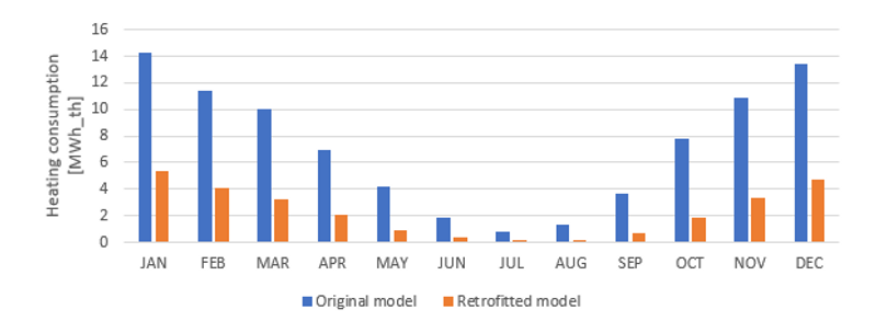
The last step in this strategy, after assessing different retrofit options, was to assign the model with the optimum retrofit measures, in order to run the simulation and deduce the total heating demand reduction. The graph below shows the heating demand of the original model against the retrofitted model.

​

​

​

​

​

​

​

 

                                                   

​

​

Figure 6: Heating consumption of original ESP-r model vs the retrofitted model.

 

The original heating consumption of the model before any retrofit measures were assigned to the model was 86.7 MWh and after implementing the complete retrofit strategy it fell to 26.9 MWh. Hence it was calculated that there was a 68% decrease in the overall heating consumption of Thomas Graham for a one-year period. The new revised energy use intensity per month was also calculated from the results generated and is shown in figure 7.

​

​

​

​

​

​

​

​

​

​

​

                                                           

Figure 7: Monthly energy use intensity for ESP-r fully retrofitted model.

​

Based on the data represented on the bar chart above, the theoretical annual heating consumption of the total floor area of the building was estimated. The following graph represents the original heating consumption of the building from heat-metered data and the theoretical heating consumption of the building that can be established when the two retrofit options discussed above were implemented. In addition, a weekly profile during winter was also generated to better visualise the demand reduction during peak periods (figure 9). Moreover, it shows the effect of simple controls in the model to regulate the time schedule of the building’s operation times. 

​

​

​

​

​

​

​

​

​

​

​

Figure 8: Original consumption of Thomas Graham vs theoretical consumption after retrofit measures.

​

​

​

​

​

​

​

​

​

​

​

                                        Figure 9: Weekly heating consumption in January for original vs retrofitted building.

​

Lastly, the total energy use intensity of the whole building was estimated to be reduced to 93 kWh/m² after escalating the results from the simulations to accommodate the difference in floor area. Referring to CIBSE guide F it was stated that the typical benchmark of EUI for a similar functionality building such as Thomas Graham should be around 110 kWh/m², which the building now meets with its revised estimated consumption. 

 

CO2 savings

​

Another key performance indicator other than lowering the demand was to analyse its effect on the CO2 emissions that can be saved after improving the energy performance of the buildings on the campus. From this strategy the analysis performed on Thomas Graham was used as an example to estimate the amount of CO2 emissions that were saved when the overall demand was decreased. The emission factor that was used was for natural gas since it is the source of energy that provides the heating to buildings across the campus. The carbon emission factor used to estimate the savings is 0.184 kg of CO2/kWh consumed (GOV.UK, 2021). From the analysis above it was concluded that with retrofitting the whole building, there was a reduction in the heating consumption by 2.1 GWh. By applying the emission factor, it was found out that in total approximately 390 tons of CO2 could be saved per annum from retrofitting only Thomas Graham as shown on figure 10. 

 

 

​

 

 

 

​

​

​

​

                                       

 Figure 10: Comparison chart for CO2 emissions before and after retrofit measures implementation.

​

 

Capital cost 

 

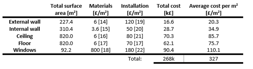
The total capital cost that the university would need to invest in retrofitting Thomas Graham was calculated based on the cost of materials and installation. To be able to proceed with costing, the total areas required for insulation or window optimisations where recorded and are summarised in the table below in addition with the prices for materials and installation. Multiple sources were considered when calculating the capital cost the values are summarised on the table below.  

 

Table 5: Overall costing of retrofitting case model

​

​

​

​

 

 

 

 

 

 

From the table above it was calculated that the average cost was £327 for every square meter that is fully retrofitted. Therefore, the final step was to calculate the estimated total cost (capital cost) for retrofitting the total floor area of Thomas Graham. From a simple multiplication between average cost and the total floor area of the building it was calculated that the total cost was around £4.5 million. 

​

 

Conclusion 

To sum up, the strategy analysis described briefly above demonstrates the effect of optimising the existing constructions of the buildings in the campus, to achieve an improved energy performance. The study was focused on one building, Thomas Graham, and based on the analysis and the results, it was found that almost a 70% decrease in the heating consumption can be achieved if these specific retrofit options are considered. As a result, it was concluded that on average a 30 kg reduction in CO2 can be established per square meter of retrofit measures implementation. In addition, this huge reduction will eventually allow the drop in the supply temperatures from the DHN which will then enable the transition from the 3rd generation district heating system currently installed to more efficient 4th or even 5th generation DHN. Moreover, an average cost of implementation per square metre of £330 was deduced, which can be used to roughly estimate the overall cost of retrofitting other buildings in the campus. Lastly from a simple investigation on the energy profiles prior and after the COVID-19 pandemic, it was identified that the university has inadequate building energy management systems which suggest a big area of improvement. By implementing such systems to the buildings not only it will manage to reduce their energy bills but also it will aim to a higher integrity of the energy system since everything will be monitored and hence any faults will be identified at an early stage. 

​

References    

​

• Charter Institution of Building Services Engineers (2015) Analytics of building management systems for improved energy and plant performance. Guide H: Building controls systems. 

• Charter Institution of Building Services Engineers (2015). Guide A: Environmental design 

• Charter Institution of Building Services Engineers (2019). Guide F: Energy efficiency

• Checkatrade (2021).  Floor insulation cost guide. Available at: https://www.checkatrade.com/blog/cost-guides/floor-insulation-cost/ [Accessed 26 April 2022]. [17] 

• Cheng, C. and Dasheng, L., (2018). Return on investment of building energy management system: A review. International Journal of Energy Research, 42(13), pp.4034-4053.

• Design buildings, (2021). Building energy management systems BEMS.1(16). Available at: https://www.designingbuildings.co.uk/wiki/Building_energy_management_systems_BEMS [Accessed 23 April 2022]. Doubleglazing-pro.co.uk, (2022). How Much do Replacement Windows Cost in 2022. Available at: https://www.doubleglazing-pro.co.uk/how-much-do-replacement-windows-cost-in-2022/ [Accessed 8 April 2022]. [22]

• Dulac, J., Peter, G., Ksenia, P. and Brian, D., (2016). Towards zero-emission efficient and resilient buildings. Global Status Report. Global Alliance for Buildings and Construction (GABC).

• Eder, P. and Delgado, L., (2006). Analysis of the life cycle environmental impacts related to the final consumption of the EU-25. Environmental Impact of Products (EIPRO). EUROPEAN COMINSION. Available at: https://ec.europa.eu/environment/ipp/pdf/eipro_report.pdf [Accessed 17 April 2022].

• Energy.gov, (2022). Update or Replace Windows.  Available at: https://www.energy.gov/energysaver/update-or-replace-windows [Accessed 7 April 2022].

• GOV.UK, (2022), Average heating degree days Available at: HEATING DEGREE DAYS .xlsx [Accessed 18 March 2022

• Homehow.co.uk, (2021). Double Glazing Cost 2022: Average Price of Double Glazing.  Available at: https://www.homehow.co.uk/costs/double-glazing [Accessed 26 April 2022]. [18]

• HomeLogic, (2019). Wall Insulation Cost Per Square Foot On Average.  Available at: https://www.homelogic.co.uk/solved-wall-insulation-cost-per-square-foot-on-average [Accessed 26 April 2022]. [15]

• Ideal Home, (2022). How much does external wall insulation cost? A full breakdown. Available at: https://www.idealhome.co.uk/property-advice/external-wall-insulation-cost-301312 [Accessed 26 April 2022]. [19]

• Insulation-info.co.uk, (2018). Roof insulation: materials & cost per square metre | insulation-info.co.uk.  Available at: https://www.insulation-info.co.uk/roof-insulation [Accessed 26 April 2022]. [16]

• Insulation-info.co.uk, (2018). Roof insulation: materials & cost per square metre | insulation-info.co.uk.  Available at: https://www.insulation-info.co.uk/roof-insulation [Accessed 8 May 2022]. [21]

• Insulation-info.co.uk, (2020). Internal wall insulation: Procedure & Pricing guidelines. Available at: https://www.insulation-info.co.uk/wall-insulation/internal-wall-insulation [Accessed 5 May 2022]. [20]

• Isidore, E., (2019). Materials. Sustainable Construction Technologies, 1, pp.237-262. Available at: https://www.sciencedirect.com/science/article/pii/B9780128117491000079 [Accessed 15 April 2022].

• Kwan, Y. and Guan, L., (2015). Design a Zero Energy House in Brisbane, Australia. Procedia Engineering, 121, pp.604-611.

• Parry, R., (2022). How much does external wall insulation cost? A full breakdown.  Ideal Home. Available at: https://www.idealhome.co.uk/property-advice/external-wall-insulation-cost-301312 [Accessed 26 April 2022]. [14]

• Strath.ac.uk, (2022). ESP-r | University of Strathclyde. Available at: https://www.strath.ac.uk/research/energysystemsresearchunit/applications/esp-r/ [Accessed 9 pril 2022].

• TWS, (2021). Air-filled vs argon-filled windows - TWS Leeds. Available at: https://www.twsleeds.co.uk/blog/air-filled-vs-argon-filled-windows [Accessed 4 March 2022].

​

Additional Information

​

                     

                    Case model geometrical and operational parameters

​

​

​

 

 

 

 

 

​
 

​

  

 

​
 

​

​

​